

4. Statistical Reasoning
Introduction and NHST
Johnny van Doorn
University of Amsterdam
2025-09-09
In this lecture we aim to:
- Introduce the S in SSR
- Repeat some stats concepts from RMS
- “Logic” behind common hypothesis testing
- Four scenario’s in statistical decision making
Reading: Chapters 1, 2, 3
Learning
About SSR
- Book: Discovering Statistics Using JASP
- Many pages, but light content
- Difficulty indications in each section (A/B/C/D)
- Theory in first half, application in JASP in second half
- Companion website of book - Data sets
About SSR
- Lectures:
- Slightly erratic
- Starts with conceptual understanding
- Ends with JASP demonstration
- Confused?
- Read the chapter first
- Rewatch lecture
- Ask questions (during lecture, on discussion board)
About SSR
- Practice:
- Tutorials, WA in Ans
- Smart Alex tasks
- Labcoat Leni examples
- Self-tests
Software
- JASP: main tool for analyses, data management
- Freely available at www.jasp-stats.org
- Also available at libraries, apps.uva.nl
- R: very flexible, 100% optional
- Freely available at https://cran.r-project.org/
- Want a nicer environment for coding? Try Rstudio
- Will be available during exam, but not required to use (can also use Ans calculator)
- Free intro course
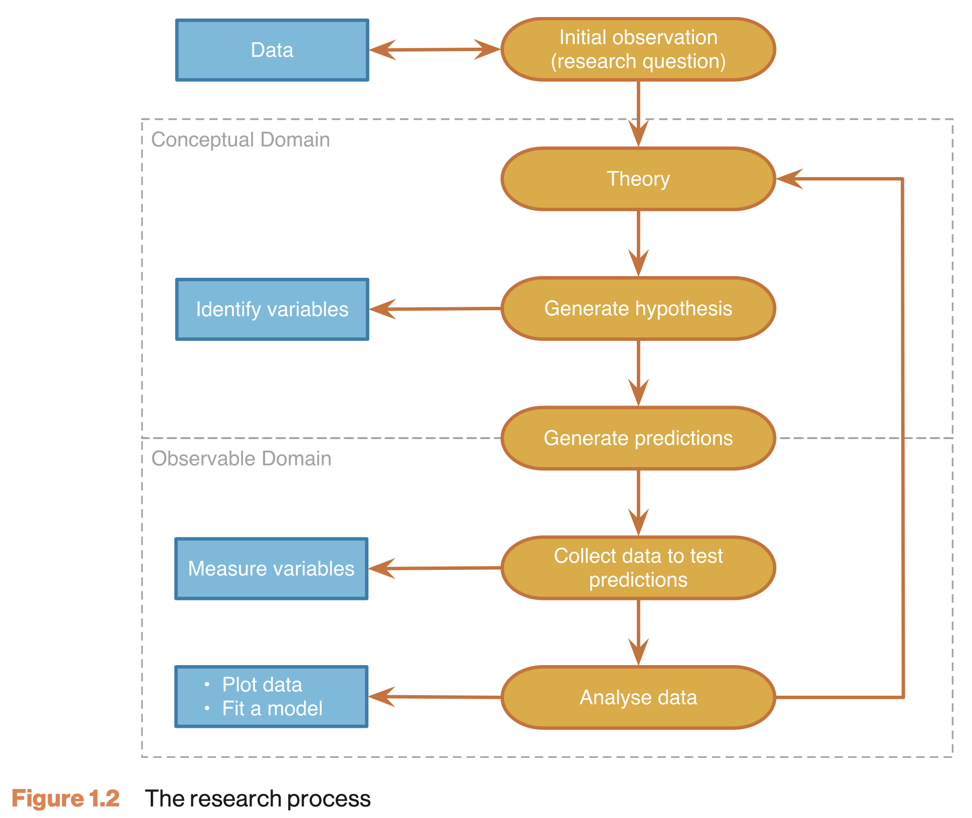
The Research Process
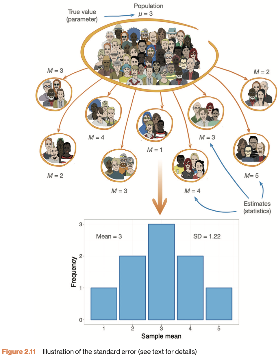
Sampling Variability
Null Hypothesis
Significance Testing
Neyman-Pearson Paradigm
Two hypotheses
\(H_0\)
- Skeptical point of view
- No effect
- No preference
- No correlation
- No difference
\(H_A\)
- Refute Skepticism
- Effect
- Preference
- Correlation
- Difference
Frequentist probability
- Objective Probability
- Relative frequency in the long run
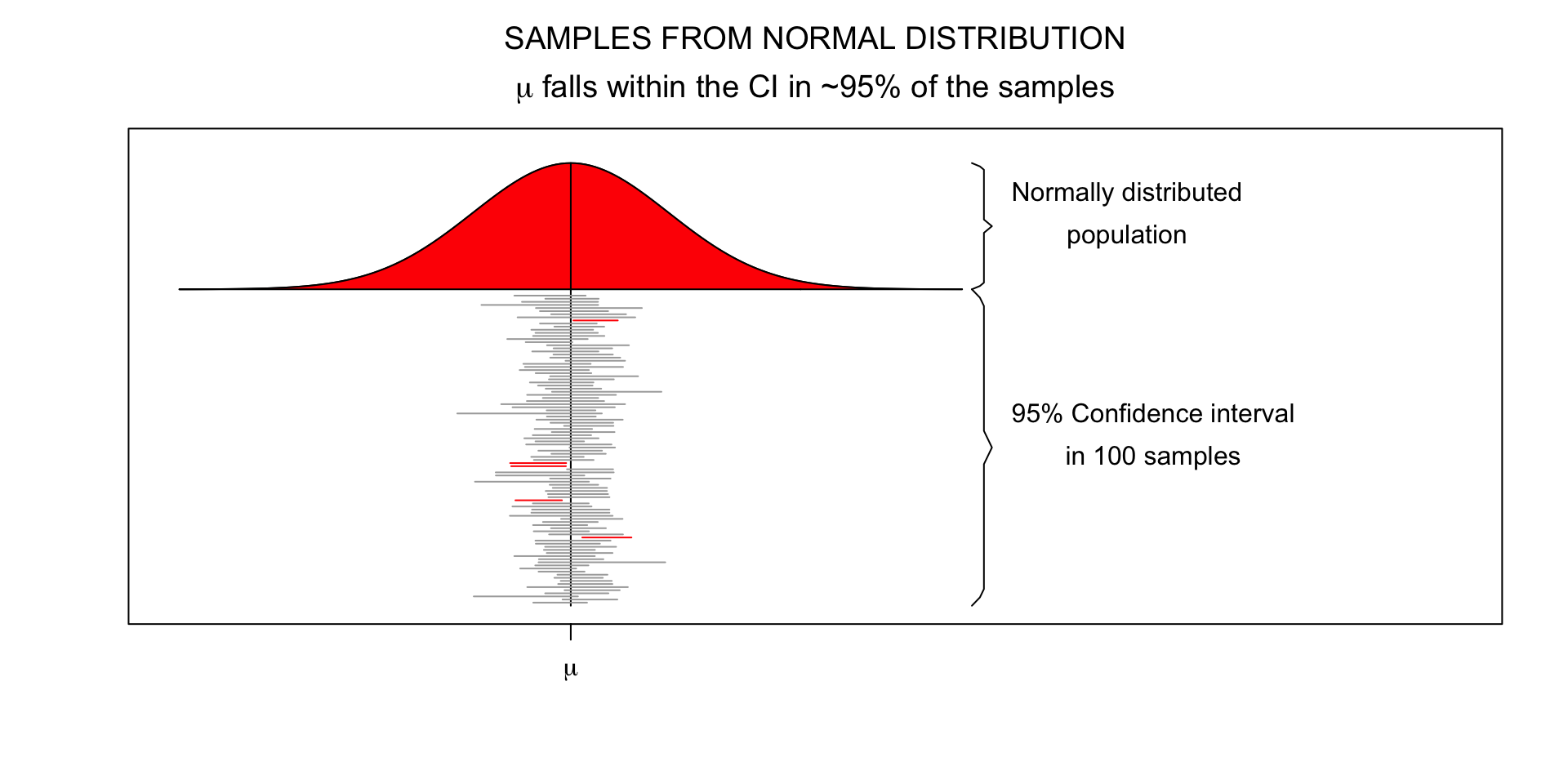
Standard Error
95% confidence interval
\[SE = \frac{\text{Standard deviation}}{\text{Square root of sample size}} = \frac{s}{\sqrt{n}}\]
- Lowerbound = \(\bar{x} - 1.96 \times SE\)
- Upperbound = \(\bar{x} + 1.96 \times SE\)
Standard Error
- n₁ =
- n₂ =
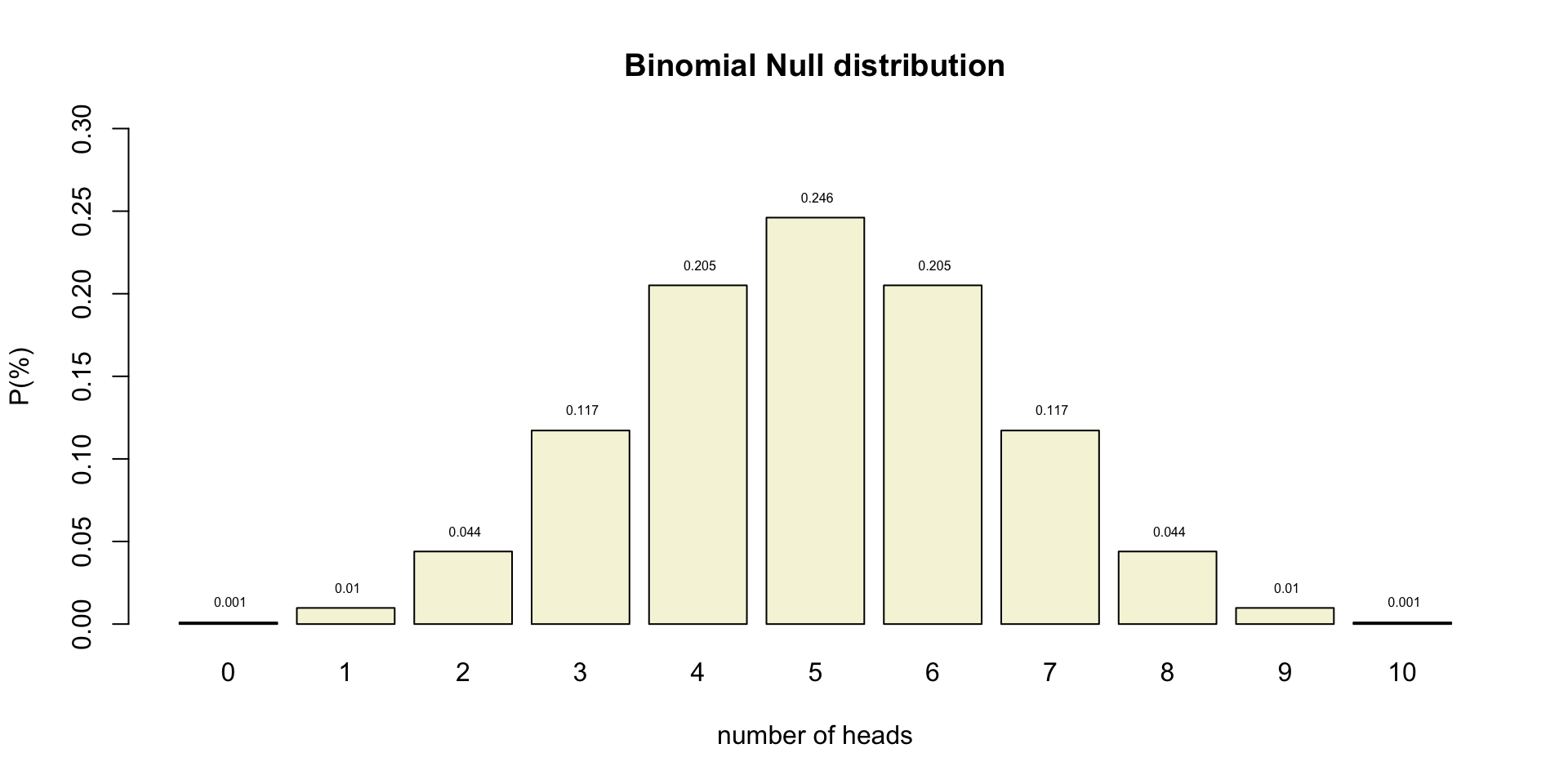
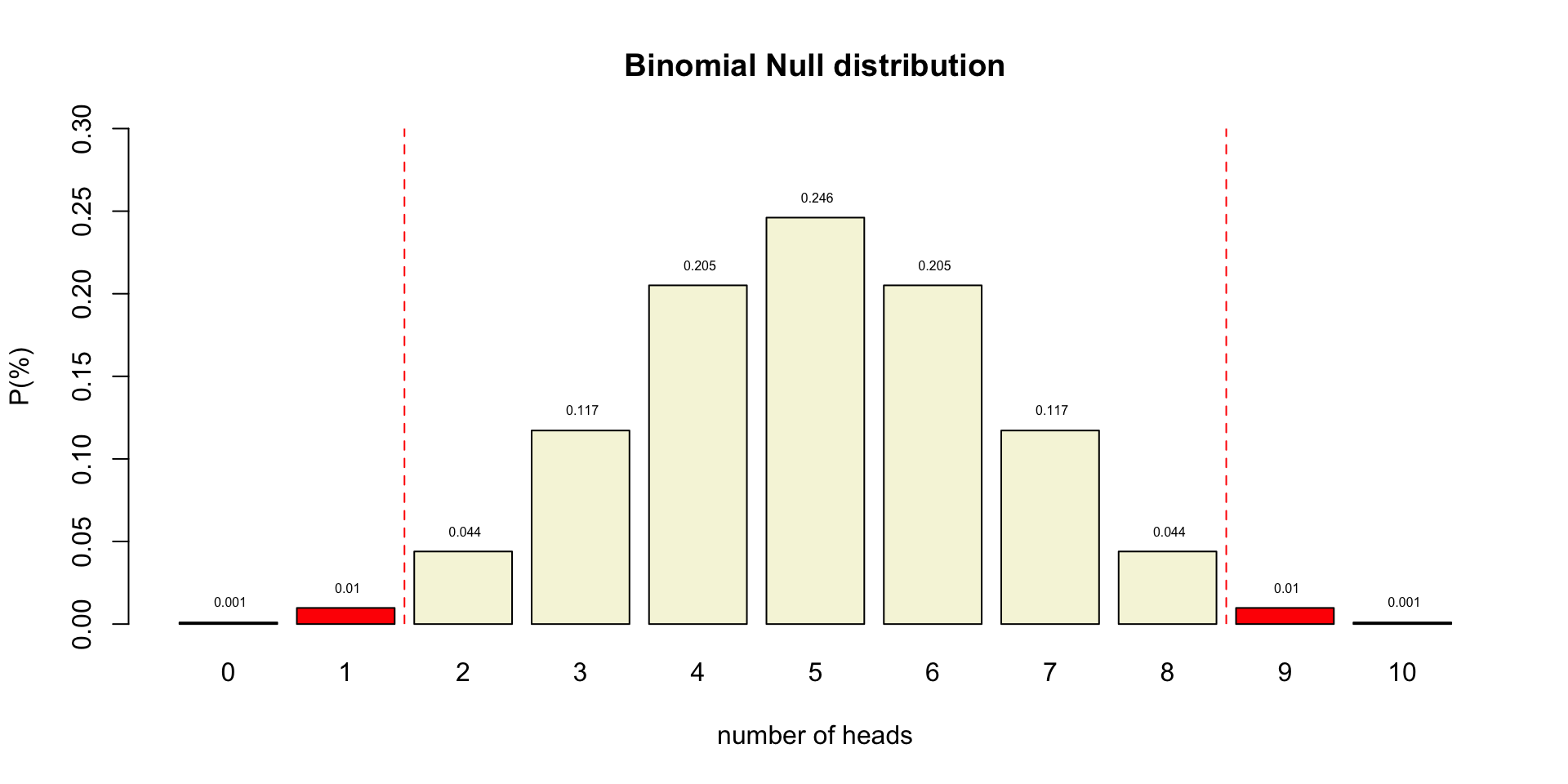
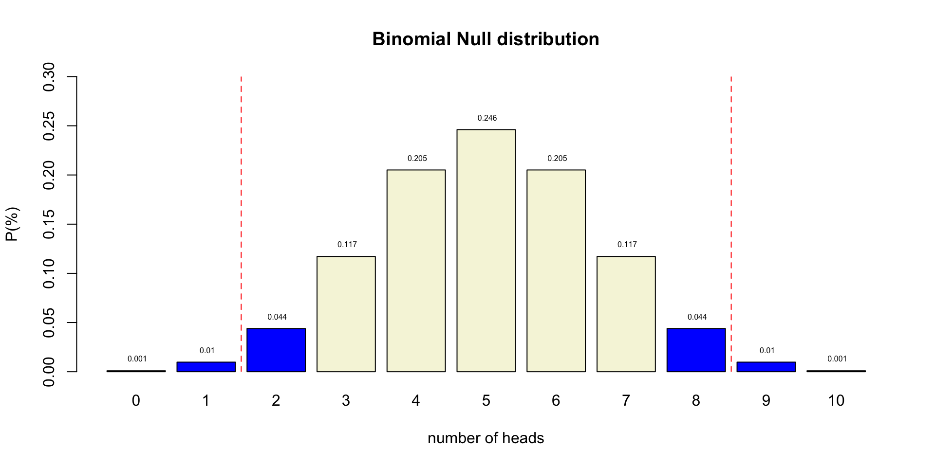
Binomial \(H_0\) distribution
n <- 10   # Sample size
k <- 0:n  # Discrete probability space
p <- .5   # Probability of head

coin <- 0:1

permutations <- factorial(n) / ( factorial(k) * factorial(n-k) )
# permutations

p_k  <- p^k * (1-p)^(n-k)  # Probability of single event
p_kp <- p_k * permutations # Probability of event times
# the occurrence of that event

title <- "Binomial Null distribution"

# col=c(rep("red",2),rep("beige",7),rep("red",2))

barplot( p_kp,
         main=title,
         names.arg=0:n,
         xlab="number of heads",
         ylab="P(%)",
         col='beige',
         ylim=c(0,.3) )

# abline(v = c(2.5,10.9), lty=2, col='red')

text(.6:10.6*1.2,p_kp,round(p_kp,3),pos=3,cex=.5)
Binomial \(H_0\) distribution
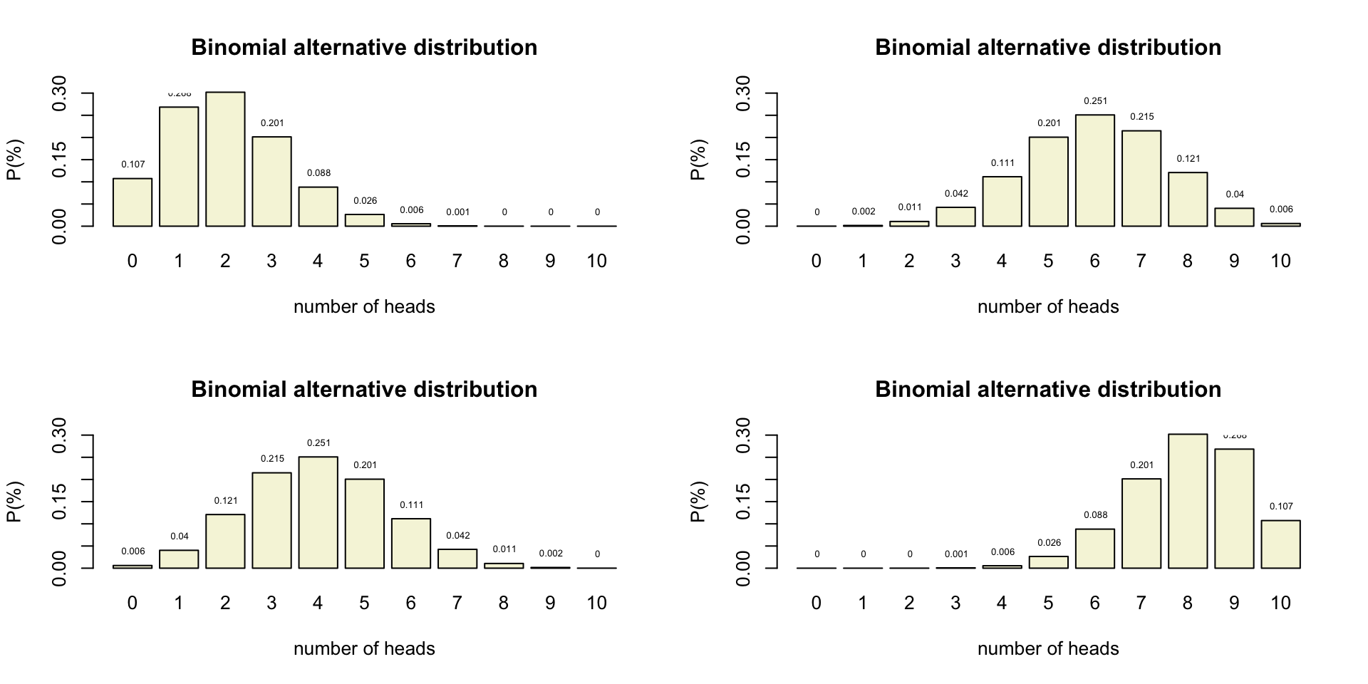
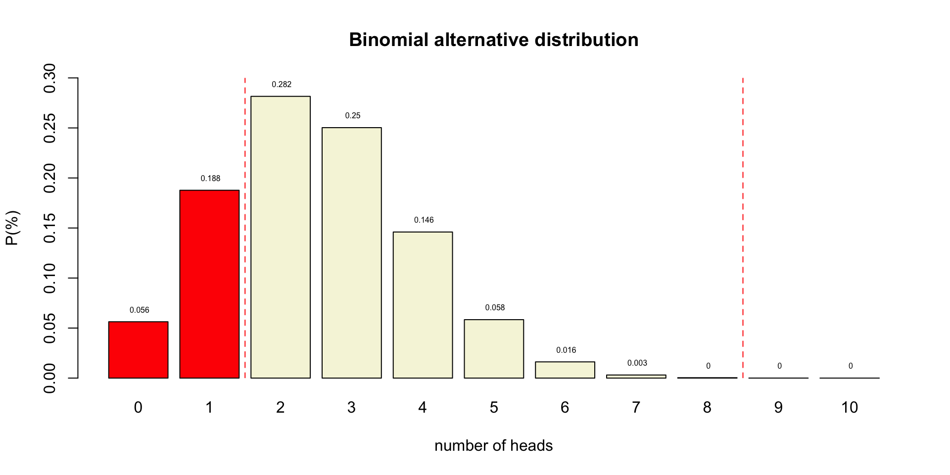
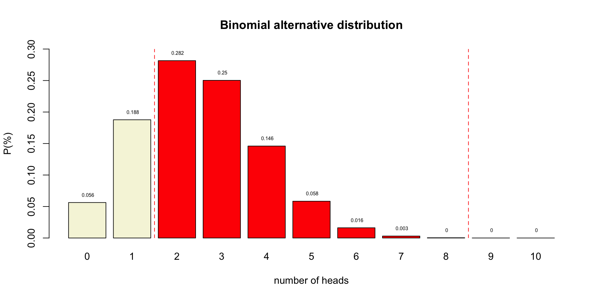
Binomial \(H_A\) distributions
Decision table
Alpha \(\alpha\)
- Incorrectly reject \(H_0\)
- Type I error
- False Positive
- Threshold for “significance”
- Criteria often 5% but heavily criticized
Power
- Correctly reject \(H_0\)
- True positive
- Power equal to: 1 - Beta
- Beta is Type II error
- Criteria often 80%
- Depends on sample size
One minus alpha
- Correctly accept \(H_0\)
- True negative
Beta
- Incorrectly accept \(H_0\)
- Type II error
- False Negative
- Criteria often 20%
- Distribution depends on sample size
P-value
Conditional probability of the observed test statistic or more extreme assuming the null hypothesis is true.
Reject \(H_0\) when:
- \(p\)-value \(\leq\) \(\alpha\)
Test statistics
A statistic that summarizes the data and is used for hypothesis testing, because we know how it’s distributed under different hypotheses
Common test statistics:
- Number of heads
- Sum of dice
- \(t\)-statistic
- \(F\)-statistic
- \(\chi^2\)-statistic
- etc…
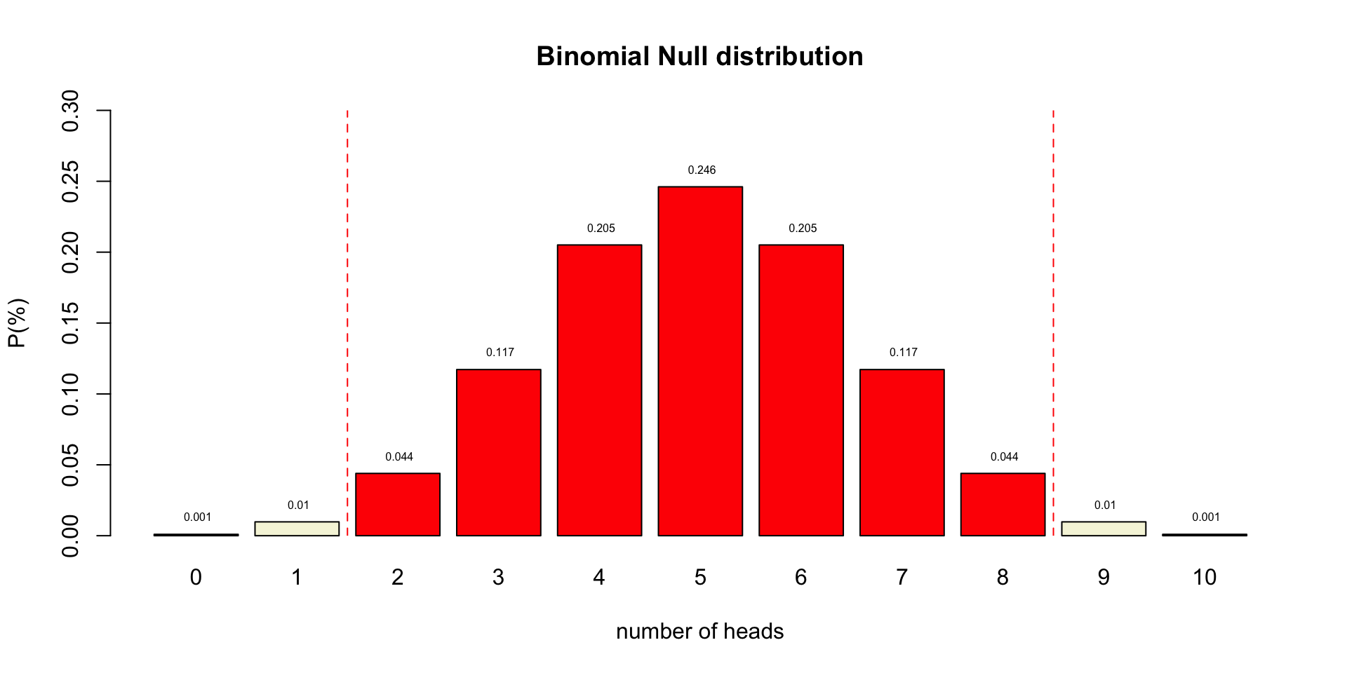
P-value in \(H_{0}\) distribution
P-value and \(\alpha\)
Alpha determines how willingly we reject the null hypothesis:
- Increase \(\alpha\) = reject null hypothesis more often
- Increases Type I error rate
- Decreases Type II error rate
- Historically set to 0.05, but widely criticized (see Jane Superbrain 3.1)
No scientific worker has a fixed level of significance at which from year to year, and in all circumstances, he rejects hypotheses; he rather gives his mind to each particular case in the light of his evidence and his ideas. (Fisher, 1956)
Misconceptions about the p-value
- A significant result means that the effect is important
- Significance = effect size + sample size
- A non-significant result means that the null hypothesis is true
- A significant result means that the null hypothesis is false
Decision Table
Play around with this app to get an idea of the probabilities
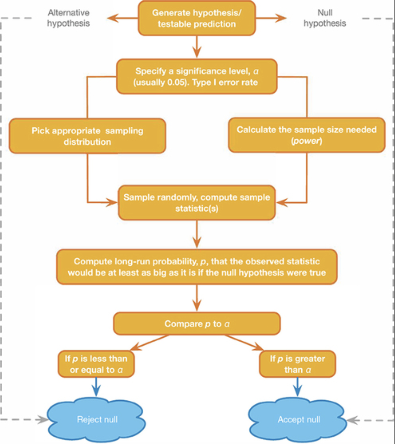
NHST Reasoning Scheme
Next Time
- Visualization in JASP
- Correlation
- How it works
- Controlling for a third variable
Bored?
Contact

![]()
Scientific & Statistical Reasoning